Showing posts with label Sheets. Show all posts

Friday, August 19, 2016

Change Row or Column Colors in Sheets


One of my favorite Google tools is Sheets. I use it for much more than just data spreadsheets. There are many tweaks that make Sheets extra cool. Conditional formatting, charts, cell formatting, and more. One of the things that is easy to do but can be labor intensive is alternating row colors for a whole sheet. The good news is that there is a quick and easy way to do this with conditional formatting! Follow the steps below to alternate colors for rows or columns in an entire spreadsheet.


Change Row or Column Colors in Sheets

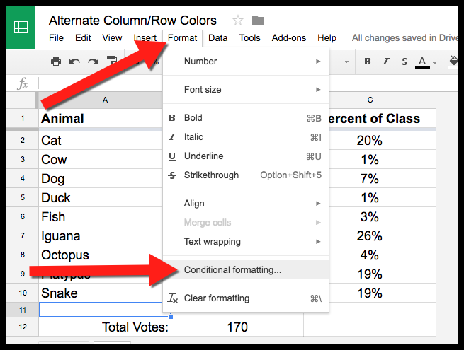
  1. In Google Sheets, click on “Format” and then click on “Conditional Formatting.

  1. Select the range using the “Apply to range” field.

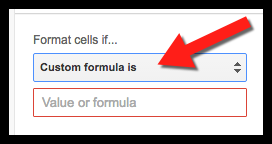
  1. Under the “Format cells if…” dropdown menu selectCustom formula is.

  1. Here is where you select which rows or columns you want to have what type of formatting (see “Apply Formatting to Rows” or “Apply Formatting to Columns” section below).
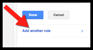
  2. After setting one row or column color click “Add another rule” at the bottom.


Apply Formatting to Rows:
  1. To apply a color to all even rows, type =ISEVEN(ROW()).

  1. To apply the rule to odd rows, type =ISODD(ROW()).

  1. Set your formatting style in the “Formatting style” box.


Apply Formatting to Columns:
  1. To apply color to all even columns, type =ISEVEN(COLUMN()).
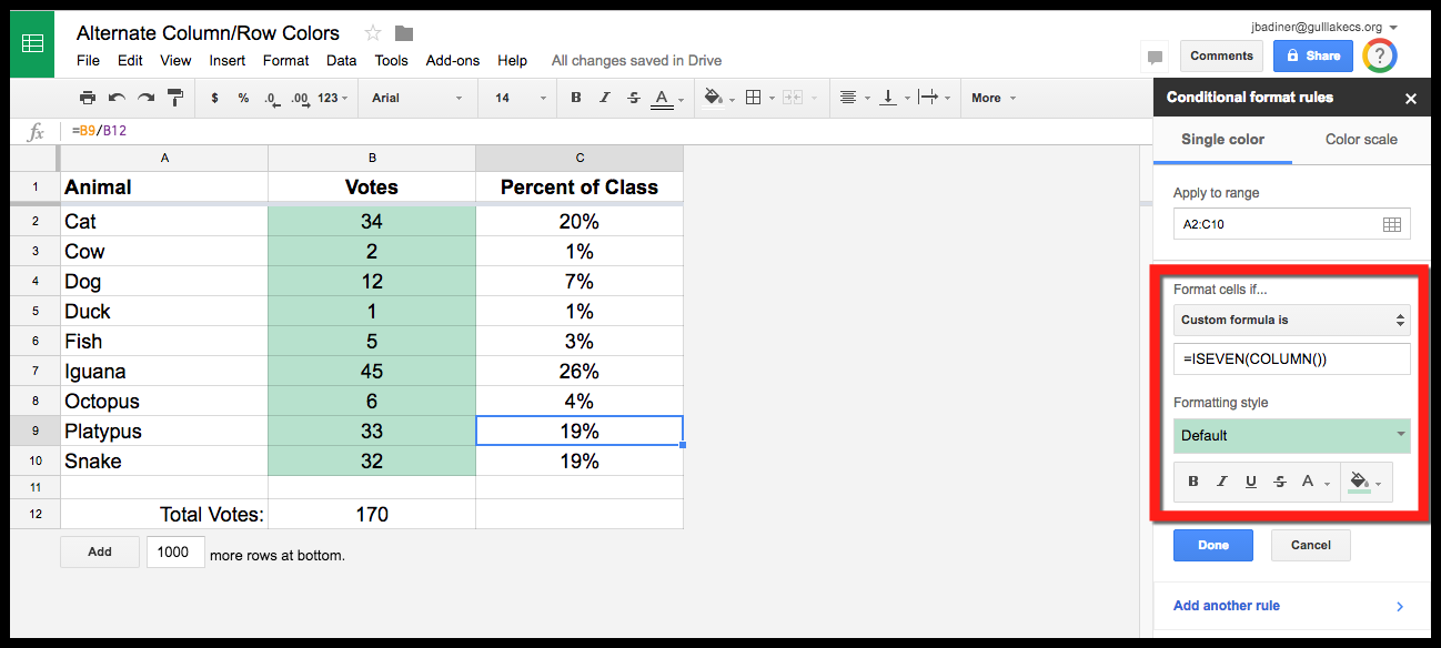

  1. To apply the rule to odd columns, type =ISODD(COLUMN()).

  1. Set your formatting style in the “Formatting style” box.


Open up a Google Sheets and give it a try!

Get these steps as a document Here!


Change Row or Column Colors in Sheets


One of my favorite Google tools is Sheets. I use it for much more than just data spreadsheets. There are many tweaks that make Sheets extra cool. Conditional formatting, charts, cell formatting, and more. One of the things that is easy to do but can be labor intensive is alternating row colors for a whole sheet. The good news is that there is a quick and easy way to do this with conditional formatting! Follow the steps below to alternate colors for rows or columns in an entire spreadsheet.


Change Row or Column Colors in Sheets

  1. In Google Sheets, click on “Format” and then click on “Conditional Formatting.

  1. Select the range using the “Apply to range” field.

  1. Under the “Format cells if…” dropdown menu selectCustom formula is.

  1. Here is where you select which rows or columns you want to have what type of formatting (see “Apply Formatting to Rows” or “Apply Formatting to Columns” section below).
  2. After setting one row or column color click “Add another rule” at the bottom.


Apply Formatting to Rows:
  1. To apply a color to all even rows, type =ISEVEN(ROW()).

  1. To apply the rule to odd rows, type =ISODD(ROW()).

  1. Set your formatting style in the “Formatting style” box.


Apply Formatting to Columns:
  1. To apply color to all even columns, type =ISEVEN(COLUMN()).


  1. To apply the rule to odd columns, type =ISODD(COLUMN()).

  1. Set your formatting style in the “Formatting style” box.


Open up a Google Sheets and give it a try!

Get these steps as a document Here!


Tuesday, June 7, 2016

Adding Charts to Slides and Docs

In a world of data we are all using charts to show classroom data. Data charts have become as common as images in our documents and presentations. The issue has been when we made these charts (using spreadsheets or other tools) we inserted them into our document or presentation and they were treated much like an image. If the data changed in the spreadsheet we had to recopy and re-insert the chart into our document or presentation. Those days are now gone! You can now insert live charts that sync to a spreadsheet and will always be up to date! Follow the steps below to learn how.


Adding Charts to Google Documents and Slides

  1. The first step (and the one you probably already have done) is to create a spreadsheet and create your chart. The chart can be anywhere within the sheet (new tab, on existing tab, multiple charts, etc).
  2. Open either a Google Document or a Google Slide.
  3. Choose where you would like the chart inserted and put your cursor there.
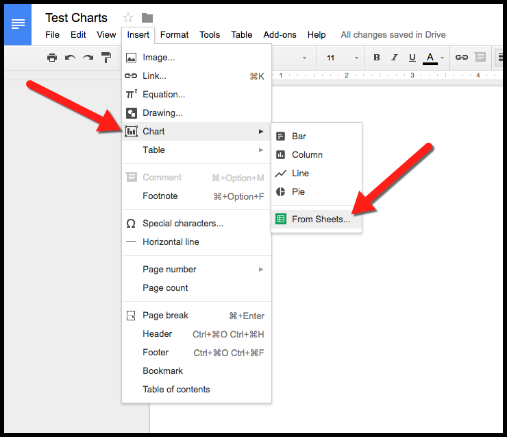
  4. Click “Insert”, choose “Chart”, and click “From Sheets”.


  1. A Drive search box will come up. Locate the Sheet that contains the chart you want and select it.
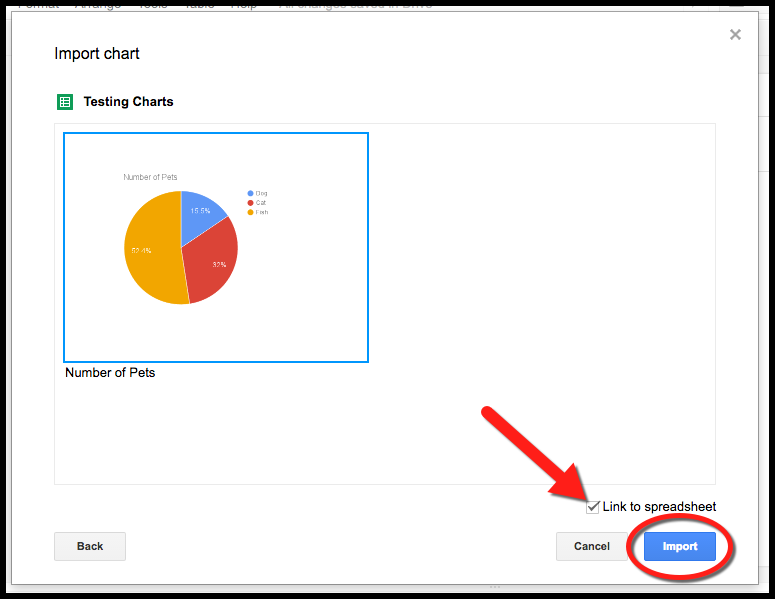
  2. The next box will show any charts that are contained within that selected Sheet. Choose the chart you want inserted into your Document or Slide.
  1. Make sure the “Link to Spreadsheet” box is selected (this will allow it to sync) and click “Import”.


  1. Resize or relocate the chart as needed in your Document or Slide.
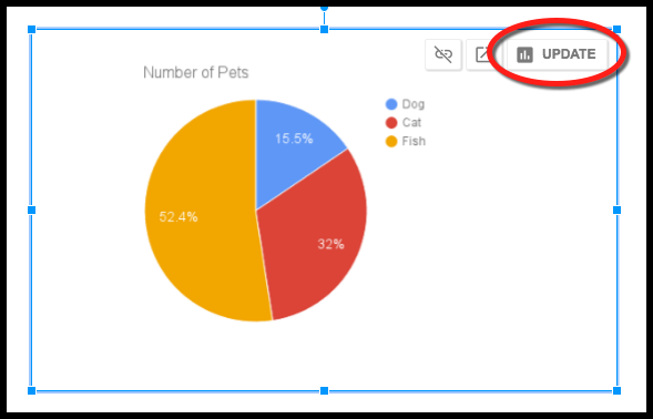
  2. If you edit the data in the spreadsheet and the chart changes, you will need to refresh your Document/Slide and click the “Update” button to make the chart update the new data.


You are all set!
Now you can keep up to date data charts working in Google Documents and Google Slides!


To see these steps in a Document, Click Here!


Saturday, November 1, 2014

miGoogle 2014: Happy Together with Google Sheets


Session Information

Abstract: Google Sheets can be used for more than just collecting and working with data. Google Sheets can be a fantastic and easy to use collaborative tool. This hands-on session will focus on some great real classroom uses for collaboration with Google Sheets such as Parent-Teacher Conference sign-up, student created vocabulary definitions, student generated book critiques, classroom party supply sign-up, student data collection/analysis, and other easy to setup and use collaborative Google Sheets. Come ready to see how Google Sheets can make your teaching life much easier!  

Skill Level: Beginner, Intermediate, Advanced

Strand: Instruction (geared for teachers) 

Featured Tools: Google Sheets, Google Drive

Time and Location: 10:10-11:00


For session location and time, please consult the printed program provided on site at the conference.


Session Resources
Please feel free to share with others. Presentation Site

Session Presenter
Jeremy Badiner is a father of 2, husband, classroom teacher (grades 3-5), Instructional Technology Coach, Google Educator, DEN Star, Common Sense Media Certified Educator (Graphite and Digital Citizenship), & ClassDojo Mentor. Oh...and a HUGE Tech Geek!